Two Criteria Lookups
In the process of teaching Excel over the past 20 years I have found that most students are often shocked and unaware that Vlookup and Index/Match can only locate the first item in a list. They find this unacceptable and I would tend to agree. When a value repeats in many rows, Microsoft suggest you use the upcoming Xlookup function to locate what is known as the ‘nth’ occurrence, but most Office365 installations will not offer that feature before July 2020 – at the earliest! For a long time there has been a workaround that does not require Xlookup, which despite Microsoft’s best intentions likely is not necessary!
In the “real world” a list typically includes items that repeat. Consider an invoice, it will typically include many line items for a single invoice number. Where one column may contain a repeating invoice number, the line items in rows could be for the same product with different size or color options. I recently came across several clients who require this functionality. While the topic of this blog post is beyond most students needs, I include it here because the class notes have finite space. This post assumes that students have taken the advanced Excel class and already understand how to work with Index and Match functions.
To follow along with the example, I recommend you download this sample workbook: Index Match Two Criteria
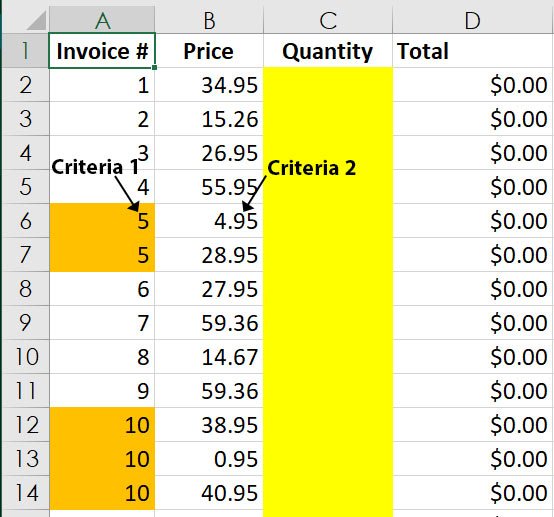
In this example notice that column A contains invoice numbers that repeat (orange cells – first criteria), and column B shows a unique price (second criteria). The goal is to locate the correct quantity for each invoiced item based on its price.

The formula required in cell C2 is:
=INDEX(DataToSearch!$F$1:$F$5061,MATCH(1,(InvoiceTwoCriteria!A2=DataToSearch!$B$1:$B$5061)*(InvoiceTwoCriteria!B2=DataToSearch!$E$1:$E$5061),0))
Given the formula’s complexity, I also recommend simplifying the readability by using named ranges, which could read:
=INDEX(Quantity,MATCH(1,(InvoiceTwoCriteria!A2=InvoiceNumber)*(InvoiceTwoCriteria!B2=Price),0))
After copying one of these formulas, take a moment to study and read it but… do not simply press the enter key, this formula requires the use of an array – hold both Ctrl+Shift while pressing the Enter key. As you study the format the formula, pay special attention to the placement of the open and close parentheses!
Because it is any array formula, we cannot reference an entire column, it requires a fixed range with absolute references (recall that named ranges are also absolute references). Also bear in mind that array formulas have limitations that can be found at this URL: https://docs.microsoft.com/en-us/office/troubleshoot/excel/arrays-limitations
The way to read and interpret the formula is:
Index (return) a value from column F. The Match lookup value of 1 creates a matrix of 1/0 values. The Match lookup array for criteria one reads: Look for the value in cell A2 (invoice #1) by searching cells B1 to B5061. The multiplication symbol before the second lookup array is treated like an AND operator. The second lookup array reads: find the price in cell B2 (34.95) by searching cells E1 to E5061. When the matrix returns a 1 match (true) for the invoice in column B, and a 1 match (true) for the price in column e, then return the corresponding value from column F (price). And if some of you are wondering, yes, this can be extended to include three criteria if needed!
If you would like to practice creating these types of formulas, download the following workbook and enable macros. Note that the submit answer feature is not expecting you use named ranges, though not incorrect the program is looking for range references, not named ranges! Index Match Two Criteria Lab

One Response